
In questo RNN Tutorial Tensorflow andremo a realizzare una rete neurale artificiale per la generazione di musica folcloristica, sfruttando la versatilità di Tensorflow e la potenza delle Recurrent Neural Network.
[google colab]
RNN Tutorial Tensorflow: Music Generation
In questo laboratorio creeremo una Recurrent Neural Network (RNN) per music generation.
Alleneremo un modello a comprendere sequenze musicali attraverso un dataset codificao secondo l’ABC notation, che usando le lettere dalla A alla G rappresenta note e altri parametri, per poi usarlo nella generazione di nuova musica!
Per prima cosa dobbiamo andare a installare alcune dipendenze.
Di queste devi sapere che la libreria mitdeeplearning, contiene il dataset che useremo per il training e la validation.
import tensorflow as tf

# Download and import the MIT 6.S191 package
!pip install mitdeeplearning
import mitdeeplearning as mdl

# Import all remaining packages
import numpy as np
import os
import time
import functools
from IPython import display as ipythondisplay
from tqdm import tqdm
!apt-get install abcmidi timidity > /dev/null 2>&1

# Check that we are using a GPU, if not switch runtimes
#   using Runtime > Change Runtime Type > GPU
assert len(tf.config.list_physical_devices('GPU')) > 0
Dataset: Data Exploration
Come ti anticipavo, il dataset è contenuto nella libreria del MIT. Contiene migliaia di melodie della tradizione irlandese, rappresentate in Notazione ABC.
Ora?
Data Exploration!
Vediamo con cosa abbiamo a che fare!
# Download the dataset
songs = mdl.lab1.load_training_data()

# Print one of the songs to inspect it in greater detail!
example_song = songs[0]
print("\nExample song: ")
print(example_song)

''' Output:
Found 816 songs in text

Example song:
[...]
B2BG c2cA|d^cde f2 (3def|g2gf gbag|fdcA G2:|!
Possiamo facilmente convertire una melodia in notazione ABC in formato audio e riprodurla, sebbene questo processo possa richiedere tempo.
# Convert the ABC notation to audio file and listen to it
mdl.lab1.play_song(example_song)
Ora, una precisazione.
La notazione ABC non si limita a rappresentare note musicali: contiene molte più informazioni.
Il titolo, il testo e persino il tempo musicale.
Quando genereremo una rappresentazione numerica dei dati testuali, capiremo come la complessità influenzi il problema.
Per il momento, limitiamoci a esplorare il dataset.
# Join our list of song strings into a single string containing all songs
songs_joined = "\n\n".join(songs)

# Find all unique characters in the joined string
vocab = sorted(set(songs_joined))
print("There are", len(vocab), "unique characters in the dataset")

''' Output:
There are 83 unique characters in the dataset
Data Processing
Quindi, giusto per ricapitolare.
Vogliamo creare una rete neurale ricorrente (RNN) per riconoscere pattern in musica ABC e usare il modello per generare (i.e. prevedere) un nuovo frammento musicale.
A un livello più profondo, quello che stiamo effettivamente chiedendo al modello è qulcosa di simile:
“Dato un carattere, o una sequenza di caratteri, qual è il successivo con la più alta probabilità?“
Benissimo, alleneremo un modello per risolvere questo task.
Conoscendo il funzionamento delle Recurrent Neural Network (RNN), forniremo alla rete una sequenza di caratteri e alleneremo il modello a prevedere il carattere successivo a ogni time step.
Avremo bisogno di un sistema che tenga in memoria gli elementi esaminati in modo che in ogni istante la rete consideri la totalità delle informazioni e non un frammento di esse.
Sento odore di struttura LSTM…
Vettorizzazione
Prima di allenare la nostra rete, dobbiamo creare una rappresentazione numerica dei caratteri; nello specifico questo significa inizializzare due tabelle di ricerca (lookup table), una che mappi sequenze di carattere in numeri e l’altra che faccia la mappatura inversa.
### Define numerical representation of text ###

# Create a mapping from character to unique index.
# For example, to get the index of the character "d",
#   we can evaluate `char2idx["d"]`.
char2idx = {u:i for i, u in enumerate(vocab)}

# Create a mapping from indices to characters. This is
#   the inverse of char2idx and allows us to convert back
#   from unique index to the character in our vocabulary.
idx2char = np.array(vocab)
In questo modo abbiamo creato una rappresentazione numerica per ogni carattere. Il nostro vocabolario è costituito da tutti i caratteri che compaiono almeno una volta, e dal relativo numero di codifica.
print('{')
for char,_ in zip(char2idx, range(20)):
    print('  {:4s}: {:3d},'.format(repr(char), char2idx[char]))
print('  ...\n}')

''' Output:
{
  '\n':   0,
  ' ' :   1,
  '!' :   2,
  '"' :   3,
  '#' :   4,
  "'" :   5,
  ...
}
Creiamo una funzione che si occupi della vettorizzazione.
### Vectorize the songs string ###

def vectorize_string(string):
  '''A function to convert the string to a vectorized
      (i.e., numeric) representation. Convert from vocab
      characters to the corresponding indices.

    The output of the `vectorize_string` function
    is a np.array with `N` elements, where `N` is
    the number of characters in the input string
  '''
  vectorized_output = np.array([char2idx[char] for char in string])
  return vectorized_output

vectorized_songs = vectorize_string(songs_joined)
Ora possiamo vedere come funziona la nostra funzione:
print ('{} ---- characters mapped to int ----> {}'.format(repr(songs_joined[:10]), vectorized_songs[:10]))
# check that vectorized_songs is a numpy array
assert isinstance(vectorized_songs, np.ndarray), "returned result should be a numpy array"

''' Output:
'X:2\nT:An B' ---- characters mapped to int ----> [49 22 14  0 45 22 26 69  1 27]
Training Examples and Targets
Ok capitano.
Ammainiamo le vele, siamo pronti a salpare.
Un’ultima cosa prima di lasciare il porto alle spalle.
Dobbiamo definire la strategia di training.
Devi sapere infatti che è nostro compito dividere il testo in sequenze che useremo effettivamente durante l’allenamento.
Ogni sequenza in ingresso conterrà un numero di caratteri pari a diciamo seq_length = 4. Dobbiamo però disporre anche della corrispondete sequenza target che avrà la stessa lunghezza di quella in ingresso, benché sia spostata, in questo caso, di un carattere.
Quindi la parola Hello sarà divisa in due frammenti:
Training Example: Hell
Target Example: ello
Questa finestra di lettura, di dimensione arbitraria, influenza le prestazioni del modello e vedremo in seguito come.
Per il momento limitiamoci a creare una funzione che crei blocchi di testi
### Batch definition to create training examples ###

def get_batch(vectorized_songs, seq_length, batch_size):
  # the length of the vectorized songs string
  n = vectorized_songs.shape[0] - 1
  # randomly choose the starting indices for the examples in the training batch
  idx = np.random.choice(n-seq_length, batch_size)

  # construct a list of input sequences for the training batch
  input_batch = [vectorized_songs[i: i + seq_length] for i in idx]
  # construct a list of output sequences for the training batch
  output_batch = [vectorized_songs[i+1: i + seq_length + 1] for i in idx]

  # x_batch, y_batch provide the true inputs and targets for network training
  x_batch = np.reshape(input_batch, [batch_size, seq_length])
  y_batch = np.reshape(output_batch, [batch_size, seq_length])
  return x_batch, y_batch


# Perform some simple tests to make sure your batch function is working properly!
test_args = (vectorized_songs, 10, 2)
if not mdl.lab1.test_batch_func_types(get_batch, test_args) or \
   not mdl.lab1.test_batch_func_shapes(get_batch, test_args) or \
   not mdl.lab1.test_batch_func_next_step(get_batch, test_args):
   print("======\n[FAIL] could not pass tests")
else:
   print("======\n[PASS] passed all tests!")

''' Output:
[PASS] test_batch_func_types
[PASS] test_batch_func_shapes
[PASS] test_batch_func_next_step
======
[PASS] passed all tests!
Cerchiamo di comprenderne meglio il funzionamento, smontandone l’operato.
Per ognuno dei vettori in ingresso, ogni indice è processato per singolo time step. Così al time step 0, il modello riceve l’indice del primo carattere nella sequenza e prevede quello successivo.
Al time step 1 l’operazione è iterata e la RNN considera le informazioni precedenti oltre all’input considerato.
Questo è quello che succede:
x_batch, y_batch = get_batch(vectorized_songs, seq_length=5, batch_size=1)

for i, (input_idx, target_idx) in enumerate(zip(np.squeeze(x_batch), np.squeeze(y_batch))):
    print("Step {:3d}".format(i))
    print("  input: {} ({:s})".format(input_idx, repr(idx2char[input_idx])))
    print("  expected output: {} ({:s})".format(target_idx, repr(idx2char[target_idx])))

''' Output:
Step   0
  input: 60 ('e')
  expected output: 59 ('d')
[...]
Step   4
  input: 1 (' ')
  expected output: 58 ('c')
RNN Tutorial Tensorflow: Neural Network Model
Ora siamo pronti a definire e allenare la nostra rete neurale, usando batch di frammenti di melodie.
Il modello fa uso dell’architettura LSTM che abbiamo imparato a conoscere qui. L’output finale del modello è quindi processato da un fully connected Dense layer attraverso una sofmax activation function che produce una distribuzione dalla quale prevedere il carattere successivo.
Useremo l’high level API di Keras per struttura agilmente la nostra rete:
tf.keras.layers.Embedding: input layer della prima tabella di ricerca (vettorizzazione dei caratteri) costituito dalle dimensioni specificate con l’hyper-parametroembedding_dimtf.keras.layers.LSTM: la nostra rete LSTM, con dimensioni dettate daunits=rnn_units.tf.keras.layers.Dense: l’output layer con un numero di output pari avocab_size.
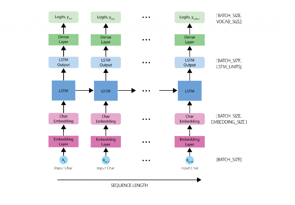
Definiamo il modello, come segue:
def LSTM(rnn_units):
  return tf.keras.layers.LSTM(
    rnn_units,
    return_sequences=True,
    recurrent_initializer='glorot_uniform',
    recurrent_activation='sigmoid',
    stateful=True,
  )
Ora usiamo la Sequential API per definire il layer del modello:
### Defining the RNN Model ###

def build_model(vocab_size, embedding_dim, rnn_units, batch_size):
  model = tf.keras.Sequential([
    # Layer 1: Embedding layer to transform indices into dense vectors
    #   of a fixed embedding size
    tf.keras.layers.Embedding(vocab_size, embedding_dim, batch_input_shape=[batch_size, None]),

    # Layer 2: LSTM with `rnn_units` number of units.
    LSTM(rnn_units),

    # Layer 3: Dense (fully-connected) layer that transforms the LSTM output
    #   into the vocabulary size.
    tf.keras.layers.Dense(vocab_size)
  ])

  return model

# Build a simple model with default hyperparameters. You will get the
#   chance to change these later.
model = build_model(len(vocab), embedding_dim=256, rnn_units=1024, batch_size=32)
Et voilla!
Il nostro modello è pronto. Facciamo un po’ di testing!
E’ una best practice assicurarci che il nostro modello funzioni secondo le aspettative eseguendo alcuni check.
Per prima cosa, eseguiamo un summary check: Model.summary stampa alcune informazioni sul funzionamento del modello. Qui possiamo verificare i vari livello della rete, l’ouput di ciascun di essi, il batch size e molto altro.
model.summary()

''' Output:

Model: "sequential"
_________________________________________________________________
Layer (type)                 Output Shape              Param #
=================================================================
embedding_1 (Embedding)      (32, None, 256)           21248
_________________________________________________________________
lstm_1 (LSTM)                (32, None, 1024)          5246976
_________________________________________________________________
dense (Dense)                (32, None, 83)            85075
=================================================================
Total params: 5,353,299
Trainable params: 5,353,299
Non-trainable params: 0
_________________________________________________________________
Possiamo anche verificare la dimensionalità del nostro output, e notare come il modello possa essere allenato usando una sequenza di lunghezza arbitraria.
x, y = get_batch(vectorized_songs, seq_length=100, batch_size=32)
pred = model(x)
print("Input shape:      ", x.shape, " # (batch_size, sequence_length)")
print("Prediction shape: ", pred.shape, "# (batch_size, sequence_length, vocab_size)")

''' Output:
Input shape:       (32, 100)  # (batch_size, sequence_length)
Prediction shape:  (32, 100, 83) # (batch_size, sequence_length, voca
Untrained Model
Per verificare le performance del nostro modello, possiamo fare una comparazione con uno non allenato. Il che equivale a considerare una previsione casuale.
sampled_indices = tf.random.categorical(pred[0], num_samples=1)
sampled_indices = tf.squeeze(sampled_indices,axis=-1).numpy()
sampled_indices

''' Output:
array([81, 71, ... 63, 51, 20])
Possiamo ora decodificare il testo:
print("Input: \n", repr("".join(idx2char[x[0]])))
print()
print("Next Char Predictions: \n", repr("".join(idx2char[sampled_indices])))

''' Output:
Input:
 "G3 BdB|AGF G2:|!\nD|GBd ... edB|AGF G2:|!\n\nX:154\nT:Tobin'"

Next Char Predictions:
 'zp"\'EI3Y!ll hi[wR!G5^ks)0>BHUlEin ... _Kc"O5MhZ8'
Beh… abbastanza senza senso.
RNN Tensorflow Tutorial Model Training
Inizia la procedura di training del modello.
Possiamo considerare il nostro un problema di classificazione, più nello specifico un multiclass-classification system.
Tante label quante i caratteri unici del testo.
Con lo stato precedente dell RNN, e l’input a ogni time step intendiamo prevedere il carattere successivo.
Per allenare il nostro modello per questo task di classificazione possiamo usare una forma dicrossentropy loss (negative log likelihood loss).
Più nello specifico andiamo a operare grazie al sparse_categorical_crossentropy loss, sfruttando la sua abilità d’impiegare valori numerici interi per task di classificazione.
Vogliamo calcolare il loss usando i target di allenamento, le label e quelle di validazione ilogit.
Calcoliamo l’errore usando le previsioni del modello randomico.
### Defining the loss function ###

def compute_loss(labels, logits):
  '''
    Define the loss function to compute and return the loss between
    the true labels and predictions (logits)
  '''
  loss = tf.keras.losses.sparse_categorical_crossentropy(labels, logits, from_logits=True)
  return loss

'''compute the loss using the true next characters from the example batch
    and the predictions from the untrained model '''
example_batch_loss = compute_loss(y,pred)

print("Prediction shape: ", pred.shape, " # (batch_size, sequence_length, vocab_size)")
print("scalar_loss:      ", example_batch_loss.numpy().mean())

''' Output:
Prediction shape:  (32, 100, 83)  # (batch_size, sequence_length, vocab_size)
scalar_loss:       4.4180417
Quindi il nostro obiettivo deve essere quello di avere un loss minore di 4.41
Definiamo una serie di hyper-parametri per il nostro modello. Quelli che trovi qui sotto sono valori ragionevoli, ma puoi liberamente modificarli per ottimizzare le performance.
### Hyperparameter setting and optimization ###

# Optimization parameters:
num_training_iterations = 1500  # Increase this to train longer
batch_size = 30  # Experiment between 1 and 64
seq_length = 250  # Experiment between 50 and 500
learning_rate = 5e-3  # Experiment between 1e-5 and 1e-1

# Model parameters:
vocab_size = len(vocab)
embedding_dim = 256
rnn_units = 1024  # Experiment between 1 and 2048

# Checkpoint location:
checkpoint_dir = './training_checkpoints'
checkpoint_prefix = os.path.join(checkpoint_dir, "my_ckpt")
Ora dobbiamo definire l’operazione di training vera e propria andando a specificare la durata dell’allenamento così come l’ottimizzatore desiderato,.
Possiamo sperimentare l’ Adam e l’Adagrad.
Riprendendo quando fatto nel precedente laboratorio, andremo prima a inizializzare il model e l’optimizer per poi usare tf.GradientTape ed eseguire la retropropagazione dell’errore.
Stamperemo infine il progresso a ogni iterazione, così da visualizzare la riduzione dell’errore.
### Define optimizer and training operation ###

'''instantiate a new model for training using the `build_model`
  function and the hyperparameters created above.'''
model = build_model(
    vocab_size,
    embedding_dim,
    rnn_units,
    batch_size
     )

'''instantiate an optimizer with its learning rate.
  Checkout the tensorflow website for a list of supported optimizers.
  https://www.tensorflow.org/api_docs/python/tf/keras/optimizers/
  Try using the Adam optimizer to start.'''
optimizer = tf.keras.optimizers.Adam(learning_rate)

@tf.function
def train_step(x, y):
  # Use tf.GradientTape()
  with tf.GradientTape() as tape:

    '''feed the current input into the model and generate predictions'''
    y_hat = model(x)

    '''compute the loss!'''
    loss = compute_loss(y, y_hat)

  # Now, compute the gradients
  ''' complete the function call for gradient computation.
      Remember that we want the gradient of the loss with respect all
      of the model parameters.
      HINT: use `model.trainable_variables` to get a list of all model
      parameters.'''
  grads = tape.gradient(loss, model.trainable_variables)

  # Apply the gradients to the optimizer so it can update the model accordingly
  optimizer.apply_gradients(zip(grads, model.trainable_variables))
  return loss

##################
# Begin training!#
##################

history = []
plotter = mdl.util.PeriodicPlotter(sec=2, xlabel='Iterations', ylabel='Loss')
if hasattr(tqdm, '_instances'): tqdm._instances.clear() # clear if it exists

for iter in tqdm(range(num_training_iterations)):

  # Grab a batch and propagate it through the network
  x_batch, y_batch = get_batch(vectorized_songs, seq_length, batch_size)
  loss = train_step(x_batch, y_batch)

  # Update the progress bar
  history.append(loss.numpy().mean())
  plotter.plot(history)

  # Update the model with the changed weights!
  if iter % 100 == 0:
    model.save_weights(checkpoint_prefix)

# Save the trained model and the weights
model.save_weights(checkpoint_prefix)
Ora possiamo impiegare la nostra neonata rete neurale per la generazione di suoni!
Prima d”iniziare dobbiamo però definire una sorta seed o seme. Una RNN non può infatti partire a freddo.
Generato il seed possiamo prevedere attraverso iterazioni successive i caratteri che compongono la notazione ABC della melodia.
Per semplificare il processo d’inferenza useremo un batch size di 1. A causa del processo attraverso cui lo stato della RNN viene passato da un time step al successivo, possiamo avere un batch size fisso.
Per modificarlo, dobbiamo inizializzare nuovamente il modello e prendere i pesi dal checkpoint precedente.
'''Rebuild the model using a batch_size=1'''
model = build_model(vocab_size, embedding_dim, rnn_units, batch_size=1)

# Restore the model weights for the last checkpoint after training
model.load_weights(tf.train.latest_checkpoint(checkpoint_dir))
model.build(tf.TensorShape([1, None]))

model.summary()

'''Output:

Model: "sequential_3"
_________________________________________________________________
Layer (type)                 Output Shape              Param #
=================================================================
embedding_3 (Embedding)      (1, None, 256)            21248
_________________________________________________________________
lstm_3 (LSTM)                (1, None, 1024)           5246976
_________________________________________________________________
dense_3 (Dense)              (1, None, 83)             85075
=================================================================
Total params: 5,353,299
Trainable params: 5,353,299
Non-trainable params: 0
RNN Tensorflow Tutorial: Prediction Procedure
Per generare un nuovo suono dobbiamo:
- definire un seed e il numero di caratteri che vogliamo generare
- otteniamo la previsione del carattere successivo a partire dalla distribuzione di probabilità
- campionare dalla distribuzione e individuare l’indice del carattere predetto
- A ogni time step lo stato della RNN aggiornato viene fornito al modello in modo che funga da contesto aggiuntivo per il miglioramento della previsione. Il processo iterativo prosegue quindi identico.
### Prediction of a generated song ###

def generate_text(model, start_string, generation_length=1000):
  # Evaluation step (generating ABC text using the learned RNN model)

  '''convert the start string to numbers (vectorize)'''
  input_eval = [char2idx[s] for s in start_string]
  input_eval = tf.expand_dims(input_eval, 0)

  # Empty string to store our results
  text_generated = []

  # Here batch size == 1
  model.reset_states()
  tqdm._instances.clear()

  for i in tqdm(range(generation_length)):
      '''evaluate the inputs and generate the next character predictions'''
      predictions = model(input_eval)

      # Remove the batch dimension
      predictions = tf.squeeze(predictions, 0)

      '''use a multinomial distribution to sample'''
      predicted_id = tf.random.categorical(predictions, num_samples=1)[-1,0].numpy()

      # Pass the prediction along with the previous hidden state
      #   as the next inputs to the model
      input_eval = tf.expand_dims([predicted_id], 0)

      '''TODO: add the predicted character to the generated text!'''
      # Hint: consider what format the prediction is in vs. the output
      text_generated.append(idx2char[predicted_id])

  return (start_string + ''.join(text_generated))

'''Use the model and the function defined above to generate ABC format text of length 1000!
    As you may notice, ABC files start with "X" - this may be a good start string.'''
generated_text = generate_text(model, start_string="A", generation_length=2000)
Il risultato finale non lo puoi vedere perché non sono riuscito a farlo partire. Onesto
Aggiornamento del 06/04/2020
Avevo commesso degli errori nel codice, ora corretti, in base ai quali l’errore era calcolato tra x e y_hat robe senza senso, e ho modificato i parametri di training del modello che risultava prima in overfitting.
Risultato?
Si chiama Dubl of the House ed è stata generata dalla RNN!
A presto!
Un caldo abbraccio, Andrea